Reverse a Cell text or Cell value

Hi All,

Today we are know about how to reverse a cell value. Means if you input "RAM" in cell A1 then it returns you "MAR" in other cell.

For doing this we make a custom function. We called the function rvrsstring.

Now, Open a new excel file then open visual basic editor by press Alt+F11 or by the following path,
Tools>macro>visual basic editor.

Now insert a new module, by Insert>module. Now paste following codes.

Public Function rvrsstring(loecell As Range, Optional istext As Boolean) Dim i As Integer Dim strnew As String Dim strold As String strold = Trim(loecell) For i = 1 To Len(strold) strnew = Mid(strold, i, 1) & strnew Next i If istext = False Then rvrsstring = CLng(strnew) Else rvrsstring = strnew End If End Function

Exit from visual basic editor and save the excel file.

Here is a sample:
Enter RAM on cell A1 and you want your result in C1 for this write a formula in cell C1 "=rvrstirng(A1,true)" this formula give you result which is "MAR".


If you want to reverse a long integer value then you can put "=rvrsstring(A1,False)"


If you put a wrong formula it shows you a error.


Here you can see a cLng commands here is a short description about cLng commands in Vba.

In Excel, the CLng function converts a value to a long integer.

The syntax for the CLng function is:

CLng(expression)

Applies To:

• Excel 2007, Excel 2003, Excel XP, Excel 2000

For more details about CLng commands you can visit the Link
Sample File: Click here

If you want to use this function on your every workbook download the following addins

Addins: Click here

Make a non printable Excel file through macro

Hi all,

Today we are discussed about how to make a non printable excel file through vba macro.

Open a new excel sheet and then open Visual basic editor by pressing alt+F11 or you also can open visual basic editor by the following path Tools>Macro>visual basic editor.
Now open Thisworkbook and copy and paste the following code on it.

Private Sub Workbook_Activate()
Dim loectrl As Office.CommandBarControl

'disable print menu
For Each loectrl In Application.CommandBars.FindControls(ID:=4)
loectrl.Enabled = False
Next loectrl

'disable print privew menu
For Each loectrl In Application.CommandBars.FindControls(ID:=109)
loectrl.Enabled = False
Next loectrl

'disable print area menu
For Each loectrl In Application.CommandBars.FindControls(ID:=30255)
loectrl.Enabled = False
Next loectrl

'disable standard print munu
For Each loectrl In Application.CommandBars.FindControls(ID:=2521)
loectrl.Enabled = False
Next loectrl

'disable set print area
For Each loectrl In Application.CommandBars.FindControls(ID:=364)
loectrl.Enabled = False
Next loectrl

' disable add to print area
For Each loectrl In Application.CommandBars.FindControls(ID:=1583)
loectrl.Enabled = False
Next loectrl

'disable exclude from print area
For Each loectrl In Application.CommandBars.FindControls(ID:=1586)
loectrl.Enabled = False
Next loectrl

'disable reset print area
For Each loectrl In Application.CommandBars.FindControls(ID:=2521)
loectrl.Enabled = False
Next loectrl

'disable page setup
For Each loectrl In Application.CommandBars.FindControls(ID:=247)
loectrl.Enabled = False
Next loectrl

End Sub

Private Sub Workbook_BeforePrint(Cancel As Boolean)
Cancel = True
End Sub

Private Sub Workbook_Deactivate()
Dim loectrl As Office.CommandBarControl

'enable print menu
For Each loectrl In Application.CommandBars.FindControls(ID:=4)
loectrl.Enabled = True
Next loectrl

'enable print privew menu
For Each loectrl In Application.CommandBars.FindControls(ID:=109)
loectrl.Enabled = True
Next loectrl

'enable print area menu
For Each loectrl In Application.CommandBars.FindControls(ID:=30255)
loectrl.Enabled = True
Next loectrl

'enable standard print munu
For Each loectrl In Application.CommandBars.FindControls(ID:=2521)
loectrl.Enabled = True
Next loectrl

'enable set print area
For Each loectrl In Application.CommandBars.FindControls(ID:=364)
loectrl.Enabled = True
Next loectrl

' enable add to print area
For Each loectrl In Application.CommandBars.FindControls(ID:=1583)
loectrl.Enabled = True
Next loectrl

'enable exclude from print area
For Each loectrl In Application.CommandBars.FindControls(ID:=1586)
loectrl.Enabled = True
Next loectrl

'enable reset print area
For Each loectrl In Application.CommandBars.FindControls(ID:=2521)
loectrl.Enabled = True
Next loectrl

'enable page setup
For Each loectrl In Application.CommandBars.FindControls(ID:=247)
loectrl.Enabled = True
Next loectrl
End Sub

Here you can see a lot of Ids and for write a code like this you must be know about all IDs. For the list of IDs click here

From the following link you can down load a sample file for the same

Download file: Click Here

Renaming the excel columns tab

Hi Friends,

Today we are discussed about how to renaming the excel columns tab label.

Actually you cant rename a columns tab in excel because excel is a spreadsheet program and you cant change the columns label.
We find a lot of questions from people how to rename a columns tab label in excel like A to "my name" column B to "my address" extra.

But due to excel is a spread sheet program you cant change the column header, for changing the columns header you must be used a database program like Microsoft Access.

But by hiding the columns header from excel you can use a excel sheets columns name you want.
For doing this you must be use the row 1 for your heading.

For hiding the columns in excel spread sheet do the following.
Go To: Tool>Option and then select view tab. Then remove the tick from the Row & Column Header. After pressing ok button you see that the row and column header are vanished from the sheet. Now in row 1 and column A you put the name which you want in this sheet.



After hide the row and columns header you put your formula like same as you put in previous.

you also can show a example of the sheet here.

Download Here

The tricky vlookup formulae

HI friends,

We are all ready know about the powerful vlookup formula in excel. I am do some test on this vlookup formula for make a master vlookup formula to lookup on the left most column from a master data sheet. I want to share the master formula with all of you.

Here is some limitation of the formula which are following:

1) In A1 cell of formula sheet put the value of A1 cell of data sheet
2) if you want to lookup on any other column then you must be change the table_array of the vlookup formula and freeze it for just one time
3)Must be put the same value in b1,c1,d1,......... which is same in the data sheet


The following vlookup formula specially describe for finding the column_index_number through the match formula


Formula Vlookup:
=VLOOKUP($A2,'Data Sheet'!$1:$65536,MATCH(C$1,'Data Sheet'!$1:$1,0),1)


here am also attached a file for showing you how you can used this formula.

if you want any clarification leave a comment me

Thank You:


Download: Click Here

Using Auto_open and Auto_close function in macro

Hi All,

First of all HAPPY DIWALI to you.

Today we are learned about two more powerful function of macro in excel.
1) Auto_Open
2)Auto_Close

1)Auto_Open: auto_open is a function in macro of excel. This function call your desired vb code before a excel workbook is open.

2)Auto_Close: auto_close is a function in macro of excel. This function call your desired vb code before a excel workbook closed.


Here am make one one example for both functions. The following are the codes.

Auto_Open function: The following code show a welcome message when ever you open the workbook in which you save the macro code. You can describe your message for the first time you open your workbook.


Sub auto_open()

ThisWorkbook.Activate

Sheets("record").Select

Range("A1").Select

txt = ActiveCell.FormulaR1C1


Do While txt = ""
txt = InputBox("You not describe any msg please write a msg.", "Welcome Message")

Range("A1").Select

ActiveCell.FormulaR1C1 = txt

If txt = "" Then

MsgBox "Please enter a msg", vbOKOnly, "Alert"

End If

Loop

ActiveWorkbook.Save

MsgBox txt, vbOKOnly, "Welcome"

End Sub


Auto_Close function: The following code show a good bye message whenever you closed the workbook on which you save the vb macro code.


Sub auto_close()

ThisWorkbook.Activate

Sheets("record").Select

Range("A2").Select

txt = ActiveCell.FormulaR1C1

Do While txt = ""
txt = InputBox("Describe a good bye msg", "Good Bye Message")

Range("A2").Select

ActiveCell.FormulaR1C1 = txt

If txt = "" Then

MsgBox "Please enter a msg", vbOKOnly, "Alert"

End If

Loop

ActiveWorkbook.Save

MsgBox txt, vbOKOnly, "Good Bye"

End Sub


Try the both code and tell me what do you think about the more powerful function in excel.
You can also download a addins of the same macro code from the following links

Download the addins: Click Here

Rename, Delete a Excel sheet by using macro

Hi All,

Today we are discussed about how to rename or delete a worksheet by using macro.

Most of the people who used excel they want to know a short cut key for renaming or deleting a worksheet

Here i am tell you how you can make a short cut key for deleting or renaming a excel worksheet by using macros.

Open a new work book and then open the visual basic editor from tools menu.

Now insert a new module for insert your code.

Now copy and paste the following codes
For renaming a sheet:

Sub renamesheet()

Dim sheetname As String

sheetname = InputBox("Enter the new sheet Name")

ActiveSheet.Name = sheetname

End Sub


For deleting a sheet with out alerts:

Sub deletesheet()

On Error GoTo msg

Application.DisplayAlerts = True

ActiveSheet.Delete

End




msg:

MsgBox "This is the last sheet in the workbook, You cant delete it", vbOKOnly,
"Alerts"

End

End Sub




save your workbook.

You also can download and use the renaming and deliting work sheet addins from the following link

Rename_delete_sheet: Click Here

Count all the comments in a active excel sheets

Hi all,

I am back again with some new excel tricks.

Today we are talking about how to count all the comments in a active excel sheet.

For doing this we use the macro. Macro is a more power full tools of excel.

For open the visual basic editor in excel do the following.

tools>macro>visual basic editor or press alt+F11

Now insert a new module from insert menu. Now copy and paste the following code under it

Sub CountComments()
commentcount = 0

For Each cell In ActiveSheet.UsedRange

On Error Resume Next

x = cell.Comment.Text

If Err = 0 Then commentcount = commentcount + 1

Next cell

MsgBox "Total Comments " & commentcount, vbOKOnly, "Sudipto Counts it"

End Sub

Now save your workbook.

from the tools menu select macro and the choose CountComments and click on options button from the window. And choose a short cut key for it, in this case i am using ctrl + m.

Insert few comments on the worksheet you want and press ctrl+m and you can see how much comments in the current active worksheet.

If you want to use the function for all of your workbook you can save your macro workbook as a addin.

For any clarification you can send me a mail.

Thank you.


Download the addins for countcomments: Click Here

Make a Task scheduler diary

Hi friends, today we are discussing about some uses of excel. Means we are going to create our simple Task scheduler. Task scheduler help us for track our imp work, like (meeting, dating, receiving family from airport etc. Now you can make your own personal task scheduler by using excel.

I am trying to making it simple. Ok let start.

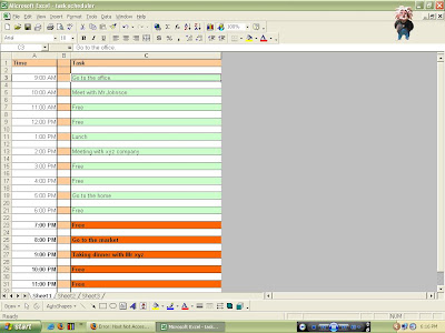
Open a new Excel workbook. Save the Excel file as a name of “task scheduler diary”, now in A1 cell write “Time”, in A3 cell write “Task” or “To Do” which is perfect for you. Now leave the second row, Put the formula in the cell A3 “=TODAY()+TIMEVALUE("9:00 am")” . Open format cells option for format cell for doing this go to format menu and then select format cells you also can open this option by using the following key combination from your keyboard “Ctrl + 1”. Now format the cell like “HH:MM AM/PM” format, for doing this follow the steps, go to number tab of the format cells dialog box then select time from category list then select “1:30 PM” from the sample list. We use this format because it is a task scheduler and we need to manage it through hourly.

Now some discussion about the formula “=TODAY()+TIMEVALUE("9:00 am")”, “=” is used because before using a function in excel it must be started with “=”. Today() commands return the current date and its time set to the 12:00 AM of the current date. Example if today is April 2, 2008 then when you give the today() command it returns “04/02/2008 00:00 AM”. “+” sign is used for sum/add. Timevalue(“9:00 AM”) returns the value of 9:00 AM in excel format. So actually our motivation is input a today value and then add 9 hour with it and it becomes 9 AM of the morning. You can set your own Task scheduler timing by changing the value of timevalue().

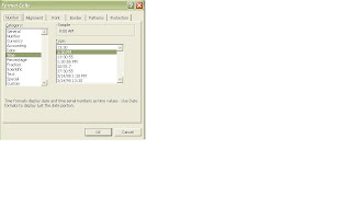
Now go to cell A4 and write the following formula on the cell “=IF(AND(A2<>"",A3="",C2<>""),A2+(1/24),"")” drag the same formula to the A33 excel change all the formula by the cell. Now select A4 to A33 range and format cells in the following format “HH:MM AM/PM”. Now discussion about the formula “=IF(AND(A2<>"",A3="",C2<>""),A2+(1/24),"")” it is a logical formula we used here the “IF” and “AND” function for conditioning. The signs <, >, =, <> are used for Less than, Greater than, Equal to, Not equal respectively. Here our motivation is If cell A2 is not equal to blank and A3 is equal to blank and C2 is not equal to blank then add (1/24) means 1:00 hour with the value of A2. Means if all the conditions are meets then one hour is add with the previous hour. Example If previous hour is 9:00 AM then the current hour is 10:00 AM.

Our Task scheduler is almost complete now it is the time for some conditional formatting with our task scheduler for a cool look. For conditional formatting select the cell C3 then open conditional formatting dialog box from the Format menu. Select “formula is” from the conditional formatting dialog box under condition 1. Then put the following formula in the formula box

“=IF(AND((A3-NOW())>=0,C3<>""),TRUE,FALSE)”, then press the format button for set the format when conditions are meet in the cell C3. Here our first condition is, If the subtraction of the value of cell A3 and current time is greater than or equal to 0 and cell C3 is not blank then the condition is true or false.

Press the add button for add a new condition name is condition 2 same here you select “formula is” from the condition 2 category. Then put the following formula in the formula box

“=IF(AND((A3-NOW())<0,c3<>""),TRUE,FALSE)”, again press the format button for format the cell when meet the following condition. Our second condition is If subtract of the value of A3 and the current time is less than zero and cell C3 is blank then condition are true.

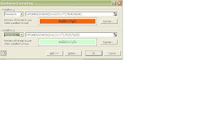
Now() command is given for show the current time and date.

Now save our Task Scheduler We just conditional formatting in the cell C3 but we need to more conditional formatting on the other cell for giving a cool look to our Task Scheduler diary. For doing this select the cell C3 and then select copy format cells by “format painter” then leave a cell below and select C5 then conditional formatting is automatically change in the cell C5 repeat the step to the cell C33 save your work.

Our Task scheduler is ready now you can save and tracking your all imp work by the task scheduler diary.

You can download a Task scheduler diary. For downloading a diary click on the following link

Task scheduler

Please send us your comments and idea for make this blog better.

How links cells of two different Excel files.

Hi friends from today we are start our tips & tricks section.

Our first topic is how links two cell by formula. For our example we first save two different files with two different names.

Let assumed name of the first file is “first.xls” and the second file name is “second.xls”.

Now first discuss about the case.

Suppose in first.xls file we have stored some detail of our customer which fields are “Name” in the column A, “Address” in the column B, “Credit price” in column C.

A B C

Name Address Credit price

In second.xls file we have stored some extra data which also include a same filed which is same with the first.xls file. The second.xls file may be look like

A B C

Customer name Product name Price

Now start our programming first we have enter some customer detail in first.xls the two same field are in the second.xls which are Name and Credit price.

We don’t want to enter the same data on both the file.

Now open the both file (first.xls, second.xls), activate second.xls window then select b2 cell then enter the formula “=[first]Sheet1!$A$2”, then drag the formula from b2 to b20(as per your requirement).

Again select C2 cell and type the formula “=[first]Sheet1!$C$2”, drag the formula from c2 to c20 (as per your requirement.

Now save both the work book and close it. Open first.xls and enter some data in it save it and close it. Open the second file what you see the data which is enter in the first cell it is automatically copy in the B and C column of the second.xls file.

Note: - Remember one thing you must be put the both file in the same directory for get the result if one of the file is missing from the directory you can not get the proper result.

You also can write a formula by doing this, put “=” in a cell then select the cell which value you want and press enter you formula is written automatically.

Moving and Copying Data and formulas in Excel

Hello friends how are you today we are learned about copying and paste feature of Excel. Actually copy and paste is not only two commands. Excel used the maximum feature of copying and paste function than the other software. So let’s start.

Copying cell contents by dragging and dropping: -

The easiest way to move or copy a cell or range of cells is to drag the cell or the range of cells to the new location and drop it.

1. Select the cell or range or range of cell you want to move.
2. Move the mouse pointer over the selections border. The pointer changes to an arrow.
3. Drag the pointer and the gray outline of the selection to the new location. Drag past the edge of a window scroll. Go to the point where you want to paste the data.
4. When you rich to the point where you want to paste the data simply release the mouse button when the gray outline is where you want to place the selected range.

To copy cell’s contents using drag and drop, do this:

1. Select the range of cells you want to copy.
2. Hold down the Ctrl key and move the pointer over an edge of the selection. The pointer becomes an arrow with a + (plus) sign.
3. Continuing holding down Ctrl key as you drag the edge of the selection to where you want the copy. The copy’s location appears enclosed by a wide gray border.

Using the drag-and-drop method, you can make only a single copy. You cannot copy to multiple locations or fill a range.

If you release the Ctrl key before you release the mouse button, the copy operation. The plus sign next to the arrow disappears. You can press Ctrl key again to switch back to copy operation.

Copying data across a Workbook:

1. Select the cell or range of cells you want to copy.
2. Click the Edit menu and choose Copy. Alternatively, click the Copy button on the standard toolbar or press Ctrl + C. The cells to copy appear, surrounded by marquee.
3. Select the worksheet to which you want to move data.
4. Select the cell at the at the top-left corner, where you want the duplicate to appear.

Using Data validation

Another great feature of Excel is data validation its validate data controls the creation of input criteria for a cell or range of cells. It can prompt a user for correct information or can display an error message if the data entered does not match the criteria.

To specify the data validation settings, do this:

1. Select a cell or range of cells for which you want to validate.
2. Click Data menu and choose validation….. .
3. In the data validation dialog box, click the settings tab property sheet.
4. Select the type of data to be validated from the Allow drop-down list.
5. Select an operator for validation from the data: drop-down list.
6. Enter the appropriate values in Minimum and Maximum: collapsable box.

To Specify an input message, do this:

1. Click the input message tab in data validation dialog box after specifying the settings property sheet.
2. Click and select the Show input message when cell is selected.
3. In the Title box enter a title for the message it is displayed in bold in the message box.
4. In the Input message: box enter a message this message is displayed below the title. The length of the message is up to 255 characters long. Press enter to start a new text in the message.
5. Click OK to save your settings.

To specify an error alert, do this:

1. Click Data menu and choose Validation…. .
2. Click the Error Alert tab in the data validation dialog box after specifying your settings property sheet.
3. Click the Show error alert after invalid data entered, so that the check box is checked.
4. Select a Style: for the message from the drop-down list.
5. Enter a title for the message in the Title: box.
6. Enter the text for the error message in the Error message: box.
7. Click OK to save your settings.

For check the criteria you select for your data validation select a cell which is under validation and then check the input message is appeared or not then enter a wrong data in this cell and press enter if error message is appeared then you success and it means which criteria you select is working.

So friends keep practicing for data validation it is very important for future use.

Auto Correct option in Excel

Excel has a great flexible feature of auto correct option which is the most important option which is commonly used in office and now those days it is used worlds wide. Auto correct will used for common typing errors and automatically corrects them as you type, it is also correct two initial capitals. You can also use Autocorrect in expand abbreviations means when you type incl, Auto automatically expand it to include. Autocorrect option is flexible because you can manage the Autocorrect option yourself.

To add AutoCorrect entries manually, do this:

1. Click the tools menu and choose AutoCorrect….. . The Auto correct dialog box appears.
2. In the replace text box, type the error or abbreviation as you usually type it.
3. In the with text box, type the correct spelling of the word or phrase or expansion of an abbreviation.
4. Click Add button to add the new entry to the list of Autocorrect entries.
5. Repeat all the steps from 2 for add more entries.
6. When you finished your work then click on the OK button.

To delete an Autocorrect entry, do this:

1. Click tools menu and choose Autocorrect….. . The Auto correct dialog box appears.
2. Select the entry you want to delete.
3. Click delete.
4. Repeat the steps from 2 how many entry you want to delete
5. When you complete your work click on the OK button.

To customize Autocorrect, do this:

1. Click the Tools menu and choose Autocorrect….. . The Autocorrect dialog box appears.
2. To turn off an option click on the check box you want to turn off the option.
3. When you finished making changes, click OK button.

Entering and Editing Data in excel

In Excel there are four distinct types of data that can reside in a cell. These types of data are:

a. Text

b. Numerals

c. Logical values

d. Error

Here we discuss about the all type of data in brief.

Text: -

The behavior of the text data are following

1. Text in a cell can contain any combination of letters, numbers, and keyboard symbols.

2. A cell can contain up to 32,000 characters.

3. If column width prevents a text string from fitting visually in a cell, the display extends over neighboring cells. However, if the neighboring cells are occupied the display is truncated.

Numerals: -

As the name of the data types it is clear that this data can contain all the decimal digits such as 0 to 9 which you ca addition, subtraction, multiplication, divides and also many mathematical and statistical calculation. We are most commonly used excel for use numerical calculation.

· Date and time are also numbers but they are in a special formatting. Let after formatting a cell if u enter 1-9 as a text string. Excel will interpret this as a date and display it as 9-jan or etc

· When a unformatted number does not fit in a cell, it is displayed in scientific notation.

· When a formatted number does not fit in a cell, number signs like hash (###) are displayed.

Logical Values: -

Excel support logical values like TRUE or FALSE in to cells. Logical values are often used in writing conditional formulas. Also there are many condition and formulas which are return logical values example if you say 3 = 4 the result is FALSE.

Error: -

It is a distinct type of data. Let in a formula you are try to divide a number by zero then the result is #DIV/0

Error value, some time when you enter a formula you can see a error which is #N/A its mean the formula is not applicable in this situation.

Date and Time in Excel

Hi friends today we are discuss about Date and Time format in Excel. Excel automatically understands date and time typed in most of the common ways. Normally when you entered a date or time in a cell Excel automatically converts it in a serial number. The serial number represents the number of days from the beginning of the century until the date you type.


If your entry is recognized as a valid date or time format you will se the date or time on screen. Correctly entered date appear in the formula bar with the format mm/dd/yyyy, regardless of how the cell is formatted.


To enter a date, do this:
1. Select the cell in which you want to enter the date.
2. Type the date into the cell with any of these formats. For example to enter a date 5th January 2008 type:
1/05/2008
05-Jan-08
05-Jan
Jan-08
Also you can enter more many types how much you can think to enter a date in Excel. And with newer version of Excel the types of entered a date format is also increased.
You must be separate a date entry with the following things /,-, or use a space to separate a date but we recommended that u must be separate with a / or -.


To Enter a Time, do this;
1. Select the cell on which you want to enter the time.
2. Type the time in any of the following formats. For example to enter 1:32 PM, type:
13:32
13:32:00
1:32 PM
1:32:00 PM
The first two examples are from a 24-hour clock. If use a 12-hour clock. Follow the time with a space and A, AM, P, PM in either upper or lower case.


To enter the current date/time in a cell, do this: -

1. To enter current date in a cell first select the cell and press Ctrl + ; keys together
2. To Enter current time in a cell first select the cell and press Ctrl + : keys together


Tips: - To format a cell in default date format, select the cell and press Ctrl + # (means Ctrl +Shift + #)
To format a cell in default time format, select the cell and press Ctrl + @ (means Ctrl +Shift +@)


Now I think all of you become expert in a date and time format of Excel. We are quickly start our one most important step which name is Formulas of Excel, it is a long lesson so friend be prepared.

Working in a workbook part III

Grouping sheets for Editing, Formatting: -

Excel gives you a great flexibility of formatting or reorganizing of your grouping sheets in workbook. That means if you have to same formatting on your three sheets then you don’t want to format the three sheets individually. You can format the three sheets simultaneously for this you must be known about the grouping of sheets. So our today’s matter of discussion is grouping worksheets.

To select a group of sheets, do this;
1) Select the first sheet tab
2) if you want to select the sheets in a adjacent then press and hold down the Shift button on your keyboard and then click on the last sheet tabs in the group the you seen the all sheet tabs between the first and the last sheet become on a group including the same. If you want to select non adjacent sheets then select the sheet first and press and hold down the Ctrl key on the keyboard and click on the other sheet, do this for each sheet tab you want to select.

To select all the sheet tabs point you mouse to the sheet tab and right click of mouse from the shortcut menu click on the Select all sheets….

Scrolling with your keyboard in Excel: -

You also know about how to scroll in Excel with your keyboard. If you think that is like moving or select a cell with you keyboard then you wrong.
For scrolling with the keyboard; do this:
To avoid change your cell selections press the Scroll Lock button on your keyboard. And then you are ready for scrolling with the key combination or individual key the list of key given following.

Key Movement direction

Up Scrolls up to one row.
Down Scrolls down one row.
Left Scrolls left one column.
Right Scrolls left one column.
PgUp Scrolls up one screen.
PgDn Scrolls down one screen.
Alt+PgUp Scrolls right one window.
Alt+PgDn Scrolls left one window.
Home Moves to the beginning of the row.
Ctrl+Home Moves to the beginning of the worksheet.



Using Go Command to move or select a cell (F5);

Hi friend this is my next lesson. I want that any person who read this blog he could understand my blog. That is not a matter he is a beginner or master in Excel. I am also trying to give you all tips.

To use the Go to command; do this:

1) Click the Edit menu and choose Go To ……or press F5. Or press Ctrl+G. The Go to dialog box appears.
2) In the Reference text box, type the cell address or range you want to go to, or select from the Go to: list box the Named location Click OK or press Enter.
3) Click Ok or press Enter.


Tips: - If you want to see the active cell, but you unable to see it in the excel window, press Ctrl+Backspace, the window scrolls to show the active cell.